|
N.B. This lab was updated on 9-13-11 for ArcGIS v. 10.0.
An older version for ArcGIS 9.2&
9.3
software can be found here. An
even older version of this lab for ArcGIS
9.1 can be found here.
4.0 Objectives
In this lab you will learn to:
-
Georeference an image
-
Create geospatial data and store it in a Geodatabase
-
Clip feature classes to a bounding box and join tables
-
Digitize in heads-up
mode, construct a topology, and edit features
4.1 Data
Data for this lab are found in the Lab_4_data folder in
the network class folder drive. They include:
- DOQQs (6, 50 cm resolution orthophotos: Art NW, NE, SE, SW and Castell NW, NE)
from
TNRIS.
These are jpeg2 format.
- Tiff image of geologic map (gat_sheet_castell.tif)
created from a partial scan of the 1:250,000 Llano Sheet of the
Bureau of Economic Geology,
Geologic Atlas of Texas. A scanned version of the map with zoom capabilities and all
collar information, including an explanation of rock units,
is also
online courtesy of the Texas Water Development Board.
A version with all collar information can be downloaded from
TNRIS at this
link. A paper copy with collar information and a legend can
also be
checked out from the Walter Geology Library.
- Roads - shapefiles for Llano and Mason Counties, and a
lookup table that contains descriptions for the road
"levels" codes. Data were created from TXDOT county
map Microstation Drawing Files, online at
TNRIS.
- Texas counties shapefile - from ESRI
- Hydrology - a shapefile (
NHD_streams_Llano.shp) of streams created from the National Hydrography
Dataset
- Hypsography - a shapefile of vector contours, from
TNRIS
- A comma delimited text file, TXunits.csv,
from the
Online Spatial Data library of the USGS containing information about the rock units on the geologic
map.
4.2 Tasks
To complete this lab you will do the following (in
order):
-
Georeference and rectify the geologic map
image
-
Create a Personal Geodatabase
-
Import the
contours, roads, county line and streams shapefiles into the Geodatabase
-
Create a Feature Dataset with a spatial domain that
encompasses the area of interest
-
Create empty feature classes within the Feature Dataset for:
-
Creates attribute fields and domains for each of the
feature classes
-
Digitize a map boundary polygon -
Digitize and attribute faults
-
Digitize and attribute point features (towns,
windmills, ranches)
-
Digitize geologic unit contacts
-
Create a contact and fault line topology
(END OF LAB 4) -
Clean the faults and contact feature classes of topological errors
(BEGINNING OF LAB 5) -
Create and attribute geology polygons
-
Clip the roads, contours and streams feature classes to the map boundary
-
Join the lookup table of road levels to the
roads feature class -
Import a roads layer file and symbolize the roads
-
Symbolize
and label the streams and contours feature classes
-
Symbolize and label geology polygons, faults and point features
-
Layout and print a map showing roads,
contours, streams, towns, ranches, windmills, faults and geological units -
Answer and turn in any questions and your layout.
4.3 Procedure
4.31 Georeferencing
-
Copy the Lab_4_data folder to your network storage.
-
Within your Lab_4_data folder, create a new folder called My_Data.
-
Open ArcMap with a new, empty document.
-
Load the 6 orthophotos from the DOQQ folder.
The spatial reference for the photos is UTM14N,
NAD83.
-
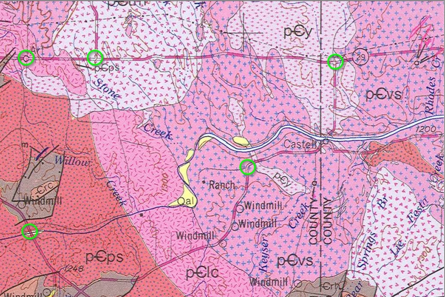
Load the scanned geologic map, gat_sheet_castell.tif.
-
Georeference the geologic map. The
image below shows suggested link points for georeferencing.
Consult the lecture notes and the
Georeferencing
Software Tip for details. For further details on
georeferencing, see pp. 317-322 in the digital book "Using
ArcMap" in the class folder (\Digital_Books\ArcMap\Using_ArcMap.pdf).
Also Search ArcGIS Help for "Georeferencing a raster dataset" and "Fundamentals for georeferencing a raster
dataset".
Watch a
short video
of part of the georeferencing process.
-
Save your georeferencing links from the Links table in your Lab4_data/My_Data folder.
-
Rectify the georefenced map, using nearest neighbor
resampling, and a cell size of 10 meters. Before
rectifying, be sure the file will be saved in your My_Data
folder.
-
Because the spatial reference of the Data
Frame is UTM14N NAD83, the rectified map should also be in
this coordinate system. Check the spatial reference of
the rectified map file before proceeding. Do
this in Arc Catalog by right-clicking on the new file and
examining the file's Properties. Forget how?
Consult
section 2.461 in Lab 2.
4.32
Creating a Personal Geodatabase and Importing
Data Files
-
Within ArcCatalog, browse to your My_Data folder,
right-click on the folder, select "New", then
Personal Geodatabase.
-
Name the new Geodatabase "Castell_Map.mdb"
-
Right-click on the Castell_Map Geodatabase icon, select
"Import", then "Feature class
(multiple)...".
-
Before importing any data, we'll first set some
"Environment" variables. This will save
some browsing/typing later. Click the "Evironments..."
button at the bottom of the window, select "Workspace", click the folder button next to
"Current Workspace", browse to your Lab_4_data
folder and click "Add". This is the only
Environmental variable we'll change, so click OK.
-
Time to Import some files... Using the folder icon
next to the "Input Features" line, browse to
your Lab_4_data folder, hold down the Shift key, and click
on the shapefiles you wish to import, i.e. both roads
shapefiles, the contour shapefile, the Texas counties
shapefile, and the streams shapefile.
Click OK and wait for the files to be imported.
-
Import the Roads lookup table (lookup_code2.dbf) using the same technique
but using right-click "Import">"Table
(single...)".
-
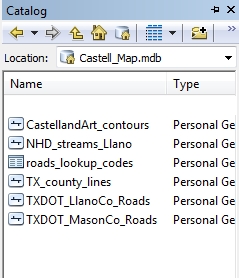
Examine the Castell_Map geodatabase in
ArcCatalog. If the above steps were completed
correctly you will see 5 feature classes and a table within the geodatabase,
as shown below.
4.33 Creating a Feature Dataset
We will need a Feature Dataset (see the lecture notes from
last week) within the geodatabase to
hold files we will create by digitizing.
Why? Without a Feature Dataset, the files we will
create could not share a topology. This is a general
rules... all files that share a topology must be contained
within the same Feature Dataset. For this reason, all
files within a Feature Dataset must have the same spatial
reference and "spatial domain" (more on this below),
which we will establish when the Feature Dataset is created.
The procedure is somewhat different for versions 9.1 and 9.3
of ArcCatalog; directions below pertain to version 10.0.
-
Right-click on your Castell_Map geodatabase, select
"New", then "Feature Dataset".
-
Name the new Feature Dataset "Geology" and
click the "Next" button to bring up the now
familiar Spatial Reference Properties window.
-
Browse to Projected Coordinate System>UTM>NAD83>NAD83 UTM
Zone 14N.prj and select (make sure the right Projected
Coordinate System is in "Name"), then click "Next".
-
In the next window you are given the chance to specify a
vertical datum. The default is none, which means that
if you have elevation information (e.g. features classes "PointZ",
"PolylineZ") that were collected with a particular elevation
datum (e.g. often NAVD88 for data collected by most GPS
units) the software will not provide a means for converting
the data to a different vertical datum. If you knew
the vertical datum for the data sets you were incorporating
this would be the opportunity to specify it. For the
purpose of this lab the default of "none" is acceptable.
-
The final window sets the "XY tolerance" (minimum distance
between between nodes or vertices before they are considered coincident).
For more on this topic, click the "About Setting Tolerance"
button. Accept the defaults and click "Finish".
4.34 Creating Feature Classes within the Feature
Dataset
We now need to create empty feature classes within the
Feature Dataset to hold the lines, points and polygons we will
digitize, as well as their attributes. Given below is
one strategy for storing the features of
this geologic map. It is not the only way this could
be done, but is relatively simple and straightforward for this fairly
simple map. A more complicated map with more features
might require a different scheme with additional feature
classes and domains.
Once the feature classes are created, we will "edit" them
to store the map features. Read about the general
process and strategies behind editing by searching ArcGIS
Help for "What is Editing?"
-
Right-click on the Geology Feature Dataset, select
"New", then "Feature Class..."
-
Name the feature class "Map_Area"
then select a "Type" for the drop down menu, in this case
the default (Polygon Features); select "Next".
-
Click the Field Name "SHAPE" to see
the "Field Properties" for the Shape field, as shown
below.
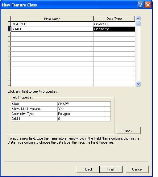
-
The "Field Properties" for the "SHAPE" field of
the attribute table for this new Feature Class (which you've
named "Map_Area") are listed in rows. The SHAPE field will
store the "Geometry Type" (in this case a Polygon representing
the footprint of the map area), coordinates, spatial
reference, and other variables of this feature class. For
more on SHAPE field property variables see pages 45-48 in
the digital book "Building a Geodatabase" or the Help files.
We don't need to change anything, nor do we need to add any
fields to the attribute table for this feature class.
-
Click "Finish". You have now created a
polygon feature class that will hold your digitized outline
of the map area. This polygon will be very useful as a
bounding box to "snap" the ends of lines to as you digitize.
We now need two new feature classes for
lines: one for faults and one for unit contacts. These
could be contained with a single feature class (both are
lines), but we will find it useful to keep them separate.
Faults can be unit contacts but may also exist within units
and "dangle", extending beyond where two units meet.
-
Repeat steps 1-3 above, using the name
"Faults" and changing the "Type" to line, then click "Next".
-
We will now add a few new fields to the attribute
table. Enter the field name "Type"
(for fault type) in the blank row below the SHAPE field
name. For future reference, Field Names can not
exceed 13 characters and can't include any special
characters, including spaces. An "Alias"
can be specified for longer names and/or coded field
names. The Data Type for this new field is
"text" and the Field Properties list should be
modified as follows:
Alias: Fault type
Length: 12 (11 characters are needed to eventually
store the values "normal", "reverse" or
"strike-slip"; 12 is overkill).
See the figure below.
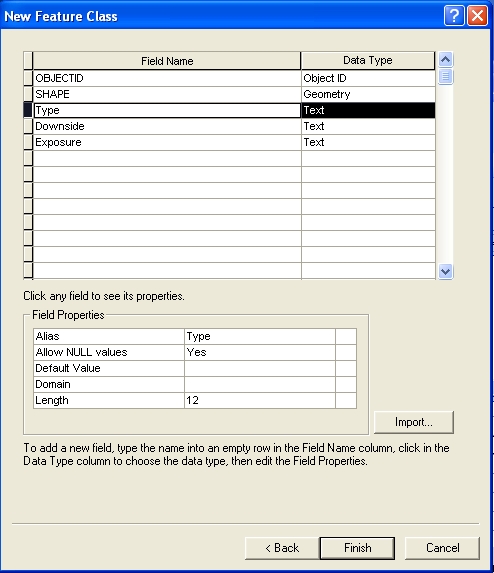
-
Repeat this process for two new text fields:
Field Name: Downside Data
Type: text
Length:3 (this will have values of N, NE, E, SE, S, SW, W,
NW, or N to indicate the down-thrown side of the fault)
Field Name: Exposure Data Type: text
Length: 10 (a field for values of Exposed, Covered,
Inferred, corresponding to solid, dotted or dashed lines
on the original map)
-
Click Finish.
Create a new line Feature Class for un-faulted contacts,
named "Contacts" following steps 1-3 and 6 above, and
using the procedure in step 7, create a new field for:
Field Name: Exposure Data Type: text
Length: 10 (a field for values of Exposed, Covered,
Inferred, corresponding to solid, dotted or dashed lines
on the original map)
-
Click Finish.
-
Create a new line Feature Class for dikes,
named "Dikes" following steps 1-3 and 6 above, and
using the procedure in step 7, create a new field for:
Field Name: Exposure Data Type: text
Length: 10 (a field for values of Exposed, Covered,
Inferred, corresponding to solid, dotted or dashed lines
on the original map)
Field Name: Rock_type Data
Type: text
Length: 25 (values are aplite,
pegmatite, marble lens)
(Note that at the scale of this map dikes (and marble
lenses) are represented as line. On a larger scale
map these might well be polygons.)
-
Create a new point Feature Class for point features,
naming it "Map_Points" with an Alias of
"Geographic Points".
-
In the drop-down menu for the SHAPE field property,
change the Geometry Type to "Point".
-
As in step 8, Add the following Fields:
Field Name:
Type Data Type:
text
Alias: Feature Type
Length: 25
Field Name: Name Data
Type: text
Alias: Feature Name
Length: 50
-
Click Finish.
4.35
Adding Domains to the Geodatabase
To avoid entry errors or repeatedly typing the same values
when "populating" the attribute tables of the
feature classes we just created, we will now define lists of
all possible attribute values for most of the fields we
created. Such lists are called
"Domains". Domains are created for the entire geodatabase, not
just for a specific feature class or feature
dataset, allowing the same domains to be used by any feature
class within the geodatabase. Once created and attached
to the feature classes, domain values can be selected from
drop-down menus in the cells of the attribute tables, a very
fast and efficient way to enter data.
-
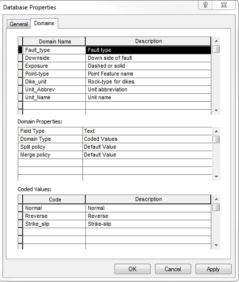
Right-click the Castell_map geodatabase icon, select
"Properties..." and click the
"Domains" tab.
-
The domains to be created have the following
names, properties and values:
| Name/Description |
Field Type |
Domain Type |
Codes/Descriptions |
| Fault_type |
Text |
Coded Values |
Normal,
Reverse, Strike-slip |
| Downside |
Text |
Coded Values |
N, NE, E, SE,
S, SW, W, NW |
| Exposure |
Text |
Coded Values |
Exposed,
Inferred, Covered |
| Point_type |
Text |
Coded Values |
Town, Ranch
House,
Windmill, Other |
| Dike_unit |
Text |
Coded Values |
Aplite,
Pegmatite, Marble lens |
|
UNIT_ABBREV |
Text |
Coded Values |
Qal, Crc, Crh,
pCyg, pCtm, pCps, pClc, pCvs |
| UNIT_NAME |
Text |
Coded Values |
Quaternary
Alluvium, Cambrian Riley Formation Cap Mt. Member,
Cambrian Riley Formation, Hickory Sandstone Member, Younger Granites,
Town Mountain Granites, Packsaddle Schist, Lost Creek
Gneiss, Valley Spring Gneiss |
All of these domains will be applied to text fields, and all will be
"Coded Value" domains, storing values as codes.
The codes are a way to speed up searching and sorting of the
final tables and have the advantage of providing drop-down
menus for data entry. But using a code different than
the "Description" produces problems when exporting
the data to ArcPad and other applications, as might be desired
if digitizing were to be done in the field. I therefore
recommend that the values entered for the Code and the
Description be identical, even though this would seemingly
defeat the main purpose of using codes. It's won't
affect searching or sorting for the small tables that we'll
create in this instance, and we won't be
exporting data in any event. Just a word to the wise for
later work.
-
Enter each of the above Domain names into a row below
the "Domain Name" heading. Leave the adjacent
"Description " column blank or type in a description of
what the domain name means.
-
Change the first two rows of the "Domain
Properties" for each domain to "Text" and
"Coded Values", respectively.
-
In the "Coded Values" area, enter the Coded
Values for each domain from the above table, using the
exact same code and description for each value. An
example for the Fault_Type Domain is shown below. The
Unit_name and Unit_Abbrev domains will be used for rock
unit polygons that we will later (Lab 6) make with ArcCatalog from the lines we digitize.
Note in the example figure below that the Coded Value for
Strike-slip is entered with an underscore, not a dash.
Coded values can not contain special characters or spaces.
-
Click OK. Other domains and coded
values can be added later, if need be.
4.36
Attaching Domains to Feature Classes
The feature classes we earlier created do not yet have
associated domains. It would seem more logical to create
the domains before creating the feature classes so that the
domains could be assigned at the same time that the feature classes
were created. This is indeed the recommended
procedure... if you have a well thought-out, preconceived database
schema!
Mine rarely are, so I usually do it the way I'm describing
here.
-
Right-click on the Contact feature class in the
geodatabase, select "Properties..." and click
the "Fields" tab.
-
Click on the Field Name "Exposure"
-
In the Field Properties area, click the blank cell to
the right of the word "Domain" to reveal a
drop-down menu; select the "Exposure" domain.
-
In the blank area to the right of "Default
Value", type Exposed. Solid lines are by far
the most common type of lines on the geologic map, thus
"Exposed" is a good default value for the
Contact Type field.
-
Notice that the software has automatically added a new
field to this feature class: "SHAPE_length",
which will be populated by the software as we draw lines.
-
Click OK.
-
Repeat steps 1-6, using the appropriate domains and
defaults, for the Faults, Dike and Map_Points feature
classes. Note that a few of the fields (e.g.
"Name") do not have domains.
Congratulations, you've now completed the
geodatabase needed for digitizing and creating the map for
this lab!
4.37 Digitizing features
Some general strategies for digitizing, otherwise known as
"Editing":
- Digitize a map boundary polygon first (e.g. the Map_Area
feature class). This polygon can be used for
clipping other feature classes to the map area and provides
a snapping target for contacts and faults.
- With snapping
turned on, digitize the same boundary with four lines saved
to "Contacts" feature class. These lines at the map
boundaries are "contacts" with the world outside the map and
will be needed to construct a topology.
-
Set Snapping before starting and check and/or reset
Snapping as new feature classes are digitized (more about
Snapping below).
Snapping is ABSOLUTELY ESSENTIAL for a result that will
not later require a lot of further editing.
- Try hard to assure that all line features that intersect
other lines are snapped to those lines or
polygons. Lines can not cross; a vertex must exist
at every line intersection.
- Work from one edge of the map to the other; examine the
map carefully and try to think a few steps ahead.
- Attribute as you go. Keep the feature class' attribute
entry window, accessible on the
editing toolbar, open as you work and fill in the fields
after completing each feature.
- SAVE YOUR EDITS OFTEN. SAVING EDITS IS DONE FROM
THE EDITING TOOLBAR, NOT FROM THE ARCMAP FILE MENU.
The editing process can crash the software more easily than
almost any other ArcMap process.
A. Digitizing the Map_Area Polygon
-
If not already open, open ArcMap and load the rectified geologic map and the
five feature classes you just finished creating (Contacts,
Faults, Dikes, Map_Area and Map_Points).
-
Check the Coordinate System of the Data
Frame. Set it to match that of the feature classes you
will edit; in this case it should be set to NAD83, UTM Zone
14N.
-
If not already open, open the Editor toolbar
(Customize>Toolbars)
-
The generalized Digitizing/Editing procedure is:
-
From the Editor toolbar menu, Start
Editing. If the Data Frame coordinate system is different
from that of the editable feature classes in your Table of
Contents, you will see the following window:
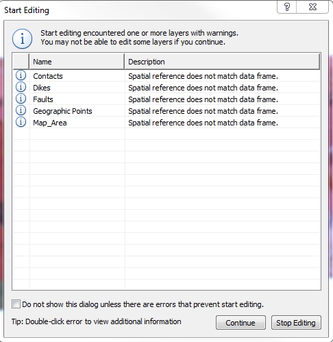
- When/If this window appears, "Stop
Editing", go to the Data Frame Properties, and change the
coordinate system to match that of the feature class you
will edit, in this case NAD83 UTM Zone 14N.
- When the Create Features window opens, select a feature
class to edit and choose a Construction Tool
Read about the Create Features window
by searching ArcGIS for "Creating features with feature
templates".
- Open the Snapping Toolbar
 (under the Editor menu on the Editor toolbar)
. (under the Editor menu on the Editor toolbar)
.
So what is this snapping business about?
See "About Snapping"
in ArcGIS 10
Help. READ THIS NOW - IT IS WELL WORTH THE TIME,
CONSIDERING WHAT FOLLOWS.
- Begin tracing or outlining a feature – create a “Sketch”
- Click to create a vertex; create vertices as needed to
outline the feature.
- Finish the feature outline with double click, or a
right-click, then "Finish Sketch";
- SAVE EDITS (on editing toolbar menu, NOT the ArcMap
toolbar).
- Open the table for the newly created feature
(table icon on edit toolbar) and enter attributes.
- SAVE EDITS.
- Repeat for the next feature.
-
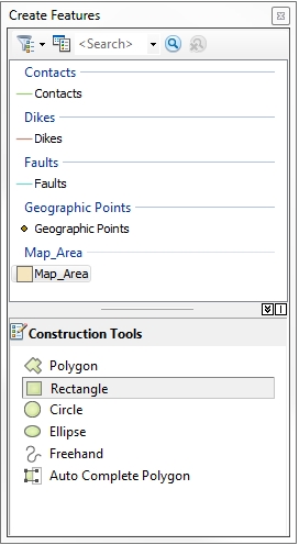
To digitize a rectangle:
- Start Editing;
- In the "Create Feature" window choose Map_Area
and the Polygon tool (as shown below);
- Open the Snapping Toolbar;
- Click on one corner of the georeferenced map,
move to another corner, then another where you finish with a
double click (or follow a single click by pressing the F2
key, or right-click and "Finish Sketch"). Don't be concerned if your polygon does
not exactly conform to the edge of the scanned map - try for
the closest fit but don't sweat it.
There are no attributes to enter for the
rectangle, so you can clear the selection (From the
Selection drop-down menu at the top of the screen, click
"Clear Selected Feature") and SAVE EDITS from the Editor
Toolbar (not the ArcMap File menu).
- Change the symbology of the new polygon to "No
Fill" with a bright green outline 1 point wide.
- Right-click on the Map_Area layer name in the table of
contents (TOC) and select "Zoom to Layer".
B. Digitizing Faults
-
If not already in Editing mode, select "Start
Editing" from the Editor drop-down menu. In the Create
Features window, click "Faults" and choose the "Line" tool.
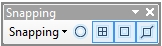
-
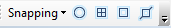
From the Editor drop-down menu select
"Snapping" to open the Snapping toolbar.
We wish to snap to the ends or vertices of other faults, and
to the edge of the Map Area polygon. Click the three
icons on the Snapping toolbar that will allow you to do so,
as shown below with the blue-highlighted icons.
Snapping is absolutely
essential when digitizing. It is impossible to
guess when a line you are digitizing is touching
another line unless you snap to it. Gaps between
lines ("undershoots") or "overshoots" can be fixed after a
topology is created, but it is much easier to get it right
the first time! -
Work from the upper left to lower right across the
map to digitize the faults. Begin by zooming into
faults that intersect the left edge of the map (a scale of
about 1:30,000 works well). Double-click to finish a
line, or right-click and "Finish Sketch" or use
the F2 key. Use vertices sparingly; most faults
are relatively straight and don't require more than a few
vertices.
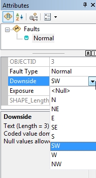
-
Click the Attributes button
 on the Editor toolbar, click a field name (e.g "Downside") and
then select the proper value from the domain values given
in the drop-down menu. An entry in progress is shown below. Do not change the OBJECTID or
SHAPE_Length values.
on the Editor toolbar, click a field name (e.g "Downside") and
then select the proper value from the domain values given
in the drop-down menu. An entry in progress is shown below. Do not change the OBJECTID or
SHAPE_Length values.
Watch a
short video
of digitizing faults. Note that the down-side
attribute is incorrect for some of the faults.
-
SAVE EDITS.
-
Use the pan and zoom tools to navigate the
map, digitizing and attributing faults as you go.
For looping faults that change trend by more than 90
degrees, there can be no one correct Downside
attribute. These should be digitized as two or more
separate faults so that each can receive a proper Downside
attribute. Likewise, topology dictates that
faults can not cross one another (geologic reasoning
dictates this too!). End the
fault you are digitizing and start a new one when the
fault you are digitizing intersects another. The new fault
should begin by snapping to the end of the fault you just
finished. Finally, all faults are presumed to be
normal faults, and the down-thrown side will always be
the side with the youngest rock unit. The ages of
the rock units can be found in the TXunits.csv file
in the Lab_4_data folder. They are also in
relative order by color in an
online version of the Llano Sheet that contains the
explanation. Some of the down-thrown
sides of faults are also symbolized with a "ball and bar".
Ask Karen if you need help.
-
To delete a fault
once it's finished, select it (using the selection tool on
the Editor toolbar), right-click and choose Delete
 . .
-
To delete or add a vertex to a completed
line, select the line with the Edit (arrowhead) tool
 on the Editor toolbar, right-click
on the line and choose "Edit vertices" (or select the
"Edit vertices tool from the Editor toolbar, or even
more simply, double-click on the line with the Edit
tool), right-click on the vertex you wish to delete and select "Delete
Vertex"; to add a vertex, right-click on the line
where you want to add one, then select "Insert
Vertex" . Vertices can be moved by dragging
while in the "Edit vertices" mode.
on the Editor toolbar, right-click
on the line and choose "Edit vertices" (or select the
"Edit vertices tool from the Editor toolbar, or even
more simply, double-click on the line with the Edit
tool), right-click on the vertex you wish to delete and select "Delete
Vertex"; to add a vertex, right-click on the line
where you want to add one, then select "Insert
Vertex" . Vertices can be moved by dragging
while in the "Edit vertices" mode.
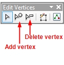
Yet another way to do this, new to ArcGIS 10.0, is with the Edit
Vertices toolbar, which is active and on-screen whenever
you are in the "Edit vertices" mode:
-
-
SAVE EDITS frequently. Once they're
saved, the program can crash and you won't loose any work.
For more on how to create and modify line
features, see "Editing vertices and segments" in the
ArcGIS Help.
-
A final word about
editing... selecting features for editing can be difficult
if more than one layer is selectable - you can
accidentally select a layer that is underneath the one
you're trying to select. To avoid this problem, the
"selectability" of layers can be turned on or off.
The easiest way to do this is by changing the TOC view to
show layer selectability, as discussed in the
last lab. Likewise, when you try to select a layer
and can't, check the Selection TOC view to see if the
layer is turned
off for selection.
Watch a
short video
of digitizing faults and adding/deleting vertices. Note that
the down-side attribute is incorrect for
the first fault digitized.
C.
Digitizing Dikes and a Marble Lens
Four
thin granite dikes, symbolized with bright red lines on the
scanned map, are
present in the NE corner of the map within the pCvs unit near
Hwy 29. Black label lines (these are not faults) connect
the letter "o" to these, indicating they are Oatman
Granite or, more generically, aplite. Similarly, a navy
blue line amongst the faults near the SW corner of the map has
a label line connected to an "m", indicating a
marble lens within the pCps unit. At the scale of
the map, these features are best digitized as single lines,
not as rock unit polygons. If you have difficulty
identifying these, look at a more legible
online version.
-
Following the procedures above, digitize
and attribute the granite dikes and marble lens.
-
SAVE EDITS.
-
Open the Attributes window and fill in the
attributes.
-
SAVE EDITS.
D.
Digitizing Map Points
Map points are the towns, ranches and windmills
on the map. They are the easiest of all features to
digitize, requiring just a single click. The map shows
the towns of Castell and Art, 4 windmills and 2 ranch houses
(as small black dots or squares).
-
In the Create Features window, choose Map_Points
(depending on whether you gave this layer an Alias e.g.
Geographic Points);
-
Click the Point tool, then click on a
point feature on the map.
-
Open the Attributes window and fill in the
attributes. If the feature is a town, type in the
name (Art or Castell), otherwise fill in the field with
Ranch or Windmill.
-
SAVE EDITS.
E.
Digitizing Rock Unit Contacts
Now for the tricky part...
Digitizing the complicated geometry of the rock unit contacts
on this map (or any geologic map) requires diligence and
attention to detail. The mechanics of the process are no
different than those just completed, however it is easy to
forget a few import details:
a) Lines can not be duplicated. They must
either start and end at other lines, or close on themselves
to become "islands", not touching any other line.
b) Lines must snap to other line edges or vertices and
can not cross. They can abut one another at a
common vertex and continue on, but they can not cross.
c) Faults and the bounding rectangle are also contacts,
the latter with the surrounding world. For
fault and map edge contacts to correspond exactly to
these features, set snapping to fault line vertices
and ends. If you trace the MAP_AREA polygon with four lines
that are within the contacts feature class, then you simply
have to snap to these lines when a contact reaches the edge
of the map. Digitize these four bounding contacts by snapping to the
vertices of the MAP_AREA polygon.
Ignore these rules at your peril. It is
very difficult (but not impossible) to construct topologically
sound rock unit polygons from digitized contact lines that
don't follow these rules.
To simplify the process somewhat, we will not
digitize the uncolored outline of the Llano River in the
eastern half of the map - simply continue lines across the
river as if it weren't there.
-
Open the Snapping toolbar (Editor toolbar,
Editor drop-down menu) and turn on Vertex, Edge and End
snapping.
-
If not already editing, select "Start
Editing" from the same menu.
-
In the Create Feature window select
"Contacts" and choose the "Line" Construction Tool.
-
Set the scale to 1:50,000, right-click on
"Layers" in the TOC, and select "Reference
Scale" then "Set Reference Scale".
You can, of course, digitize
at a larger scale but this
greatly exceeds the accuracy
of the original map and will
cost you a lot more time.
DIGITZE LINES AS THEY APPEAR
AT 1:50,000; DO NOT WASTE
TIME WITH MORE VERTICES THAN
ARE NECESSARY.
-
The first "contacts" to digitize are the
contacts of the rock units with the surrounding world,
in other words the map boundaries.
-
Set snapping to snap only to vertices .
-
Digitize a line that traces the outline of
the Map_Area polygon.
-
To digitize rock unit boundaries, turn
snapping for edges and ends back on, begin in the NW corner and work Eastward
and Southward, digitizing lines, snapping to the boundary
or other lines, and attributing as you go. Actually,
you should not have to do any attributing if the default
for "Exposure" is set to "Exposed" - these are all solid
lines. Get comfortable, this will take some time...
-
If you make mistakes, see the procedure
above
for removing or adding vertices, and for deleting lines.
-
SAVE EDITS often.
Watch a
short video
of digitizing contacts.
4.38
Create a Topology for the Map
Lines
Before creating rock unit polygons from the
Map_Area, Contact and Fault lines, it is useful to
"clean" the lines of errors that will corrupt
polygon creation. This is most easily (?) done by
creating a topology layer in the Geology feature dataset that
contains rules designed to spot errors. After setting up
the rules and creating the topology, the topology can be
"validated", and explicit violations of the rules
will be flagged for easy editing.
-
From the ArcCatalog window within ArcMap (or from
ArcCatalog program), right-click on the Geology feature
dataset, select "New", then
"Topology". The Topology wizard opens.
-
Click "Next", accept the name the new
topology ("Geology_Topology"), and change the cluster
tolerance to 15 (15 meters; see the description of cluster
tolerance).
-
Click "Next" and place a check in
the boxes adjacent to the "Contacts"
and "Faults" feature classes
- these are the feature
classes we are checking for dangling and/or crossing lines.
-
Click "Next" and change the
number of ranks to 2. Change the rank for Contacts
to 2; this will allow Contact line nodes to move rather
than faults (they should stay relatively straight lines)
if snapping is done during the creation of the topology.
-
Click "Next" to bring up the
topology rules dialog. We need rules for both
contacts and faults. As already stated, we want to
know where contact lines dangle (not meeting other contact
lines) and where they cross themselves.
We'd also like to know the latter for faults.
a) Click the "Add Rule..." button and,
for the Contacts feature class, select the rule (from the
drop-down menu) "Must Not Overlap".
b) Repeat step a), this time choosing "Must Not
Have Dangles".
c) Repeat step a), this time choosing
"Must Not Self-Intersect".
d) Repeat steps a) and c) for the Faults feature
class. Do not repeat step b) for Faults; faults are
allowed to dangle.
For a nice explanation of all available topology rules,
search "Geodatabase topology rules and topology error fixes"
in ArcGIS Help.
-
Click "Next" and review a
summary of Topology properties.
-
Click "Finish" and wait for the
Topology feature class to be created. Answer
"Yes" to Validate the topology now.
-
A new feature class has been created that
contains flags for every rules violation. Some of
these may be valid exceptions to rules, others
are errors. To see the violations, preview the
topology feature class in ArcCatalog by right-clicking on
the new file, selecting "Item Description" and then the "Preview" tab. The pink squares
are the locations of errors, which we will later view on
top of contacts feature class in ArcMap. To get a list of errors,
right-click on the topology layer, select
"Properties", click the "Error" tab
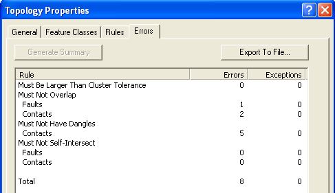
and click the "Generate Summary" button.
If you've done a careful job of
digitizing and snapping, your Summary might look something like the one
shown below. The Summary shows 3 errors for the
"Must not overlap" rule and 5 for the "Must not have
dangles". Yours may be better (wouldn't that be
great) or worse (ugh).
End of Digitizing Part 1 (Lab 4)
In Part II of this Lab (Lab 5, next
week) we will go through and
fix the errors before going on to make
rock unit polygons, attribute them, and complete the map.
|
|