I. Introduction
During today's lab you will create
topographic and aerial photographic maps that you will later use for geologic
mapping. The maps will be created from digital images of four, 7.5 minute
topographic quadrangles (Digital Raster Graphs;
DRGs), and from portions of four digital aerial photographs (orthophotographs;
DOQs). The software you will use to
merge and overlay the images is E.S.R.I.'s
ArcInfo 9.0, a suite of powerful G.I.S. tools that, among other things, is designed to
manipulate georeferenced vector- and raster-based maps and images. In lab today
you will:
- Become familiar with the cartographic
features of ArcInfo 9.0.
- Construct and manipulate layers of images
and other data.
- Build and layout a printable map.
II. The Data
Digital data for today's lab come from the
Texas Natural Resources Information System ( TNRIS)
who, via the web, distribute
DRGs and DOQs for the entire state, for free. Texas is in the forefront of distributing such data, and TNRIS is a
national leader. DOQs are available at several
resolutions; your data have individual pixels that image 1 square meter of ground.
The DRG and DOQ images are stored and organized by 7.5 minute USGS quadrangle names and by lat./long.. DRGs are the
scanned equivalents of single, 7.5
minute quadrangles, including all collar information (scale bar, N arrow,
graticules, etc.), that have been reprojected to a UTM projection and stored as
TIFF files that are ~ 5-15 Mb in
size. Most recently, TNRIS has made these available without collar, permitting
much easier tiling of multiple maps. The four DRGs we will use today were
downloaded without collars, making our job of producing a single map from them
much easier.
DOQ images are distortion-free,
uniform-scale, color infrared aerial photographs that cover slightly more than a
quarter of each 7.5 minute quadrangle, (called Digital Orthophoto Quarter
Quads., or DOQQs). The quarter quad. photo size is necessary to keep file sizes
manageable; a full, 1 meter resolution DOQQ is about 150 Mb when stored in
(uncompressed) Tiff format. Most recently these files have been made available
in MrSID format, at very
higher compression ratios. Files are still quite large for all but
state-of-the-art computers, so for this lab, file size has been further reduced
by trimming the DOQQs to only the mapping area and immediate surroundings.
The map we will make overlaps the junction of four adjacent 7.5 minute quadrangles. By name, these
are Long Mountain, Sheep Run Creek, Turtle Creek and Long Mountain. Their
relative locations are indicated below.
|
long_mt |
grit |
| sheep_run_ cr |
turtle_cr |
To be useful for GIS purposes, DOQQs and
DRGs must contain a reference to their geographic location and scale. So-called
"georeference data" for DRG and DOQ images are stored in small text files of the
same name, but with .TFW extensions. TFW files contain UTM coordinates for the top right corner of each
image, as well as information about the size of the pixels, allowing precise
registration of all images and accurate on-screen coordinates. Both DRGs and
DOQQs are UTM projections but are not mapped on the same datum; DRGs, like their
paper counterparts, are mapped on the NAD 27 datum and DOQs on NAD 83. With
proper care, ArcInfo software can account for these differences, permitting
perfect registration and overlay, despite differences in datums.
III. The Software
We will only use some of the cartographic
features of ArcInfo in today's lab. As a GIS tool, the program has many other
powerful features we will not explore. Those interested in learning more can
examine tutorials available through the
E.S.R.I. web site, or visit the
Geo327G lab pages.
Data in ArcInfo 9 is organizes into “map
documents”, so-called .mxd files, and, within map documents, by "Data Frames”.
Data Frames have "Properties", e.g. the type of map projection, the coordinate
system, measurement units, etc., can be set to match the data, or to reproject
data to a different coordinate system. Data Frames are composed of "Layers",
which can contain images, vector maps, databases or other information. Your
Data Frame will consist of several layers, including layers for DOQs and DRGs.
Layer "Properties", such as colors, line weight etc., can be adjusted.
Data Frames can be manipulated and viewed
while in “Data View” or “Layout View”. The latter provides a
what-you-see-is-what-you-get view, as it will appear when printed. UTM or other
grids, scale bars, a north arrow, text, and any other items that might be placed
in the collar of the map are visible in Layout View, but not Data View. The
printing routine is very similar to any other Windows software, as are toolbars
for adding graphics and words.
IV. The Procedure
Data for today's lab are stored in a class
folder labeled "420K" on one of the Department’s servers, geosrv, on the path
geosrv/main/course directories/420k/Lab12.
- Log onto the network (you will be provided a user ID and password) and browse to
geosrv/main/course directories/420k/Lab12. Do this with the help of the instructor.
- Create a folder on drive c: named 420K_GIS to store the data and project when completed.
- Copy the Lab12 folder from the server to 420K_GIS folder on the lab computer
(this increases access speed and avoids network sharing conflicts). Highlight,
drag and drop.
- Open your copy of the lab 12 folder and double click on the file “Lab12_basemap.mxd. This
starts the ArcMap program and opens up a previously created mxd (map document)
file that is empty except for a 100m UTM grid and some text explaining the grid
and data sources.
- Click the yellow + button
 to add layers. You will need to add the following three layer files from your Lab12 folder
(all have yellow diamond-shaped icons):
to add layers. You will need to add the following three layer files from your Lab12 folder
(all have yellow diamond-shaped icons):
- Orthophotos.lyr
- Raster Graphs.lyr
- Ranch_hypsography.lyr
- Set the map scale to 1:12,000. Do this by typing 12000 into the scale window
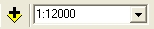 on the
toolbar.
on the
toolbar.
- If necessary, change the order of listing so that the Raster Graphs layer is on top
of the Orthophotos layer, both of which should be beneath the hypsography layer.
Do this by dragging the name of the layer in the table of contents. Themes are
turned on and off (made visible or invisible) by clicking on the box adjacent to
each theme title in the table of contents (shown here).

Each theme is a map layer, superimposed on one another in the order listed.
Turn off the photographs and the hypsography layer, leaving only the Raster
Graph layer on.
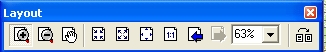
- Tools for exploring the maps (zooming, panning, refreshing, returning to the previous
view, querying, measuring) are available on floating tool bars. Very importantly, there
are two general kinds of tools that look exceedingly similar, those to use in
“data view” and those to use in “layout view. We will mainly
use tools for layout view in lab today. Using the Layout tools
(shown below), zoom, pan and
explore your maps.
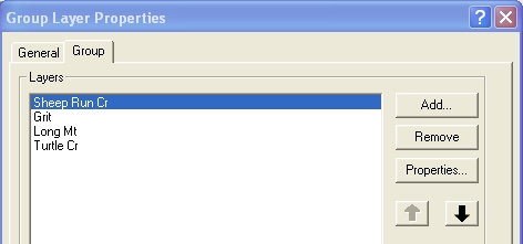
- Many functions in ArcMap are available on menus accessible by a right
mouse click on the layer name in the Table of Contents. We wish to remove
some of the colors from the raster graphs to see the photographs underneath. Right click on the
Raster Graphs layer, select “Properties..” from the menu, click the “Group” tab
(shown below),
click on one of the four layer names and click the Properties button.
Within
the Layer Properties dialog, select the Symbology tab (shown
below) and select from the colors
shown all but the blue, brown and black colors (all but colors 0, 2, 4, 8, 12). Click the Remove button, then OK.
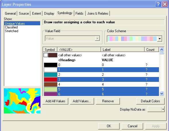
Repeat this process for the remaining three
raster graphs to allow the aerial photos to become visible.
After removing these colors from all of the DRGs, click the Apply button at the
bottom of the Group Layer Properties window, then OK.
- Turn on the Orthophotos layer. You should now be able to see the contours of the raster graph on top of the
aerial photographs. They are in the traditional brown of all USGS maps and look
somewhat pixilated, particularly at higher magnification. To
render these more visible on the photos, the brown color could be changed to
yellow or white within the Symbology tab of step
9, but this is
unnecessary, because there is a better source for contours than the raster
graphs.
- Turn off the Raster Graph layer and turn on the hypsography layer. The hypsography layer contains a very clean version of the contours from the
same four quadrangles, trimmed to the Lansford Ranch mapping area. The data
were downloaded by a somewhat complicated process from the TNRIS website while
viewing TNRIS data in ArcCatalog, a component of ArcInfo. These are vector
data (rather than raster), so they will not degrade at higher magnification.
- Insert a scale bar and some text (including your name in the upper right hand corner) using the
Insert menu at the top of the window (shown below)
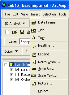 and the “new text" (A) button and the “new text" (A) button
 at the bottom
of the window. Change the scale bar parameters (by doubling clicking on the
scale bar to bring up a properties window) to make a scale bar in 100s of meters
with at least five increments.
at the bottom
of the window. Change the scale bar parameters (by doubling clicking on the
scale bar to bring up a properties window) to make a scale bar in 100s of meters
with at least five increments.
- Making sure the scale is set to 1:6000 and the map is centered on the area specified in
class, and without anything but the hypsography layer turned on, print your map
to a black and white laser printer.
- Without changing a thing, turn on the orthophotos layer and print the map to a color
laser printer somewhere in the building (the instructor will identify one for
you).
- We now need a detailed (1:3000) map of the area to be mapped on Sunday.
The mapping area is centered on 463750mE, 3401600mN. Use the hand tool from
the data frame toolbar to center you map on these coordinates. Change the scale
to 1:3000. Compare your result to that of the instructors.
- At a scale of 1:3000, centered on the coordinates above, repeat printing steps 14 and
15 above.
- Retrieve your output, put it with your gear for the field trip, and be sure to bring it
this weekend!
Back to Lab 12
|
Back to Lab 12
GIS Data |